Theory
Governing Equations
pyBaram can solve convection-diffusion equations, which are written as follows.
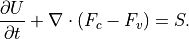
where  is the vector of conservative variables.
 are the convective and viscous flux, respectively.
 is the source vector.
Euler Equations
The governing equations of inviscid flow are written as follows.
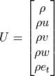
where,  is density,
  are components of velocity vector and
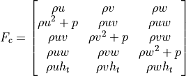
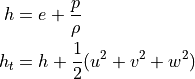
 is the total specific energy. From equation of state,
specific internal energy can be written as follows.
is the total specific energy. From equation of state,
specific internal energy can be written as follows.
where  is pressure and
  is ratio of specific heats.
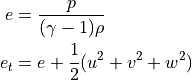
Euler equations have only convective flux, which can be written as follows.
where  is total specific enthalpy, which can be defined as follows.
Navier-Stokes Equations
Viscous flux of Navier-Stokes equations are written as follows.
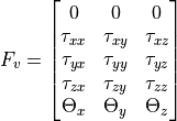
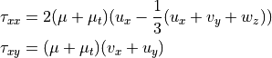
where,  is shear stress, which can be written as follows.
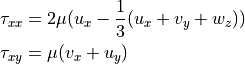
 is viscosity and
  is derivative of velocity. Other components of the stress tensor are defined analogously.
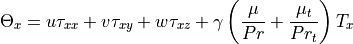
  can be written as follows.
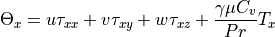
where,  is temperature and
  is Prandtl number, which is a non-dimensionalized value.
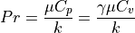
where,  is specific heat at constant pressure,
  is specific heat at constant volume and
  is thermal conductivity.
RANS Equations
For RANS (Reynolds-averaged Navier-Stokes) equations, the turbulent viscosity is computed using turbulent model equation. pyBaram employs two models: the one equation Spalart-Allmaras model and the two equation SST model. With turbulent viscosity  , shear stress in viscous flux can be modified as follows:
Turbulent thermal conductivity is computed using turbulent Prandtl number  , thus
in viscous flux can be modified as follows.
, thus
in viscous flux can be modified as follows.
Finite Volume Method
Cell-centered finite volume method is employed to discretize in space. For each cell, the semi-discrete form of the governing equation can be written as follows.
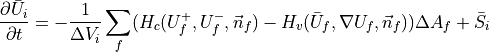
where
 and
and  represent the cell-averaged state variable vector
and source term vector at the
represent the cell-averaged state variable vector
and source term vector at the  cell, respectively.
 and
and  denote numerical inviscid and viscous fluxes, respectively.
 and
and  correspond to the face-averaged state and
gradient vectors at the
correspond to the face-averaged state and
gradient vectors at the  face, respectively.
Furthermore,
face, respectively.
Furthermore,  and
and  denote the unit normal vector and area
of the face, respectively.
denote the unit normal vector and area
of the face, respectively.  is the volume of the cell.
 and
and  are the left and right state vectors at the face;
they can be obtained by MUSCL-type reconstruction, as below
are the left and right state vectors at the face;
they can be obtained by MUSCL-type reconstruction, as below
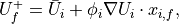
where  corresponds to the gradient of the state variables at the cell
and
corresponds to the gradient of the state variables at the cell
and  denotes the position vector from cell center to face.
Furthermore,
denotes the position vector from cell center to face.
Furthermore,  is slope limiter at i-th cell for robustly capturing shock discontinuities;
can be computed similarly at the adjacent cell.
is slope limiter at i-th cell for robustly capturing shock discontinuities;
can be computed similarly at the adjacent cell.
The procedures to compute the right-hand side can be summarized as follows:
Gradient Calculation
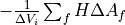
The gradient of each cell is computed by least-square, green-gauss or its hybrid [1] and numerical formulation can be written as follows.
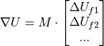
where  is pre-computed operation matrix and
  is difference of
conservative vector at f-th face of the cell.
is difference of
conservative vector at f-th face of the cell.
pyBaram computes gradient with two steps.
- Compute at each
Intersclass inpybaram.solvers.baseadvec.inters make_delu method generates loop.
construct_kernels method of each
Intersgenerates kernels.
- Compute
- Compute
 at
at BaseAdvecElementsclass inpybaram.solvers.baseadvec.elements. Operation matrix
is pre-computed at _prelsq method of BaseElementsclassmake_grad method of the class generates loop.
construct_kernels method of the class generates kernels.
- Compute
Slope Limiter
In order to capture shock-wave robustly, the slope of linear reconstruction should be limited.
pyBaram computes MLP-u slope limiter with two steps.
 at each
 MUSCL-type reconstruction
With gradient and slope limiter on each cell, the and is reconstructed linearly.
- Compute MUSCL-type reconstruction
 at each
 BaseAdvecElementsclass inpybaram.solvers.baseadvec.elements make_recon method of the class generates loop
construct_kernles method of the class initiates kernels.
- Compute MUSCL-type reconstruction
Convective Flux
Each Inters class in pybaram.solvers.euler.inters computes convective flux.
make_flux method generates loop to compute convective flux along the interface.
At construct_kernels method of the
Intersclass inpybaram.solvers.baseadvecgenerates kernels. are pre-computed and stored as _mag_snorm and _vec_snorm at
 BaseIntersclass inpybaram.solvers.base.inters.Various approximate Riemann solver
are implemented in pybaram.solvers.euler.rsolvers.fpts in each element stores
 before execution and saves
  after execution.
Viscous Flux
Each Inters class in pybaram.solvers.navierstokes computes viscous flux.
make_flux method generates loop to compute viscous flux, as well as convective flux, along the interface.
Averaged state and gradient vectors at face are computed.
Viscous flux
is implemented in pybaram.solvers.navierstokes.visflux
Negative Divergence of Fluxes
After computing flux at faces, divergence of flux can be computed with finite volume method.
- Compute
 at
at BaseAdvecElementsclass inpybaram.solvers.baseadvec.elements. _make_div_upts method of the class generates loop.
construct_kernels method of the class generates kernels.
- Compute
Turbulence Models
One or Two equations of RANS turbulence models are also computed with similar procedure. Source terms are added after divergence of flux.
Time Integration
After computing the right-hand side (negative gradient of flux), the solution can be updated through integration over time. Currently, explicit Runge-Kutta schemes [13, 14] and implicit LU-SGS schemes [15] are implemented. The classes for these integrators are provided in the pybaram.integrators module.
References
Eiji Shima, Keiichi Kitamura, and Takanori Haga. Green-gauss/weighted-least-squares hybrid gradient reconstruction for arbitrary polyhedra unstructured grids. AIAA Journal, 51:2740–2747, 11 2013. doi:10.2514/1.J052095.
Jin Seok Park, Sung Hwan Yoon, and Chongam Kim. Multi-dimensional limiting process for hyperbolic conservation laws on unstructured grids. Journal of Computational Physics, 229:788–812, 2010. URL: http://dx.doi.org/10.1016/j.jcp.2009.10.011, doi:10.1016/j.jcp.2009.10.011.
Jin Seok Park and Chongam Kim. Multi-dimensional limiting process for finite volume methods on unstructured grids. Computers and Fluids, 65:8–24, 2012. URL: http://dx.doi.org/10.1016/j.compfluid.2012.04.015, doi:10.1016/j.compfluid.2012.04.015.
Philip L Roe. Approximate riemann solvers, parameter vectors, and difference schemes. Journal of computational Physics, 135(2):250–258, 1997.
Sung Soo Kim, Chongam Kim, Oh Hyun Rho, and Seung Kyu Hong. Cures for the shock instability: development of a shock-stable roe scheme. Journal of Computational Physics, 185:342–374, 2003. doi:10.1016/S0021-9991(02)00037-2.
Seongyu Choi, Donguk Kim, Jaehyong Park, and Jin Seok Park. Robust and accurate Roe-type Riemann solver with compact stencil: Rotated-RoeM scheme. Journal of Computational Physics, 505:112913, 2024. URL: https://doi.org/10.1016/j.jcp.2024.112913.
Kyu Hong Kim, Chongam Kim, and Oh Hyun Rho. Methods for the accurate computations of hypersonic flows. i. ausmpw+ scheme. Journal of Computational Physics, 174:38–80, 2001. doi:10.1006/jcph.2001.6873.
Meng Sing Liou. A sequel to ausm, part ii: ausm+-up for all speeds. Journal of Computational Physics, 214:137–170, 2006. doi:10.1016/j.jcp.2005.09.020.
B. Einfeldt, C. D. Munz, P. L. Roe, and B. Sjögreen. On godunov-type methods near low densities. Journal of Computational Physics, 92:273–295, 1991. doi:10.1016/0021-9991(91)90211-3.
Vladimir Vasil'evich Rusanov. Calculation of interaction of non-steady shock waves with obstacles. NRC, Division of Mechanical Engineering, 1962.
Spalart P. R. and Allmaras S. R. A one-equation turbulence model for aerodynamic flows. Recherche Aerospatiale, pages 5–21, 1994. URL: https://turbmodels.larc.nasa.gov/Papers/RechAerosp_1994_SpalartAllmaras.pdf.
F. R. Menter. Two-equation eddy-viscosity turbulence models for engineering applications. AIAA Journal, 32:1598–1605, 1994. doi:10.2514/3.12149.
L Martinelli and A Jameson. Validation of a multigrid method for the reynolds averaged equations. AIAA 26th Aerospace Sciences Meeting, 1988.
Sigal Gottlieb and Chi-Wang Shu. Total variation diminishing runge-kutta schemes. Mathematics of Computation, 67:73–85, 1998. doi:10.1090/s0025-5718-98-00913-2.
Seokkwan Yoon and Antony Jameson. Lower-upper symmetric-gauss-seidel method for the euler and navier-stokes equations. AIAA Journal, 26:1025–1026, 1988. doi:10.2514/3.10007.